“There are times when you need more information than a tube tester can provide.
Matching a pair of audio tubes is one example.”Daniel Schoo: Tube testing expert, author of “Calibration of the Hickok 539C Tester” and Electronics Design Engineer at Fermilab.
Tube Testers Just Don’t Provide Enough Information
Only a curve tracer can properly perform tests such as matching a pair of audio tubes, or determining if a power tube is capable of providing its full rated output power in a particular amplifier, or determining a tube’s optimum bias setting for a certain amplifier.
Vacuum tube curve tracers are rare compared to tube testers. They are complex, expensive laboratory type instruments, and require considerable training for proper use. However, the added effort is well worth it. Unlike tube testers that can only show simple characteristic such as transconductance at only one operating point, curve tracers show you all operating parameters across all operating conditions – all at once.
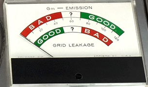
For repair work a simple test on a tube tester to find out if a particular tube is serviceable (good or bad) is sufficient. That’s what they were designed to do. But when you need detailed information about a tube’s performance under actual operating conditions, a curve tracer is the only practical way to find it. That’s what curve tracers were designed to do.
Output tubes matched for audio amplifiers should be balanced within 2% or less at their actual operating voltage and bias current. The more unbalanced tubes become, the more hum, harmonic distortion, and intermodulation distortion they produce.
When it comes to tasks like matching tubes a tube tester’s single point comparison of transconductance, plate current or other parameters is almost never correct because they are not measured at actual operating voltages and load currents.
Correctly matching tubes is greatly simplified when you can see the transconductance, plate resistance and plate current graphically represented at the tube’s actual in-amp operating range of plate and grid voltages. Additionally, with a curve tracer detailed A‐B comparisons between two tubes can be made visually with the throw of a switch.
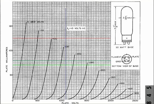
Also, the only reliable way to test a tube’s general condition or “quality” is to produce the same set of operating curves shown in the manufacturer’s data sheet. Only by using the same voltages and currents given in the curves contained in the manufacturer’s data sheet can you find the real answer to what condition the tube is in.
For a good tube, the curves should look very much like the data sheet and be very close to the values printed on its graphs. A bad or week tube will show low plate currents and weak transconductance, especially at higher operating loads. A “leaky” tube will show lines sloping downward compared to the data sheet’s curves.
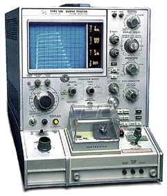
We currently use two curve tracers:
1. An “old school” Tektornics 576 manually operated tracer. It has been modified especially for audio tube curve tracing with the capability to plot transconductance and amplification factors over a wide range of grid, plate and screen voltages – up to 1,500 volts at up to 220 watts output.
2. A “new-school” uTracer model 3+ fully computerized (software driven) tracer. It has also been modified, allowing us to precisely duplicate the operating conditions of any amplifier (up to 480 volts and 50 watts per tube). It can simulate the exact grid, cathode and plate circuit conditions found in most amps, allowing us to test your tubes in their true operating environment.
Only a Lab-Quality Curve Tracer Can Really Do It
In most curve tracer graphs the vertical scale is the plate current, the horizontal scale is the plate voltage – just like the curves in a tube manual. Each curve in the set or ‘family’ of curves shows a plot of the plate current from zero to maximum operating volts on the plate for a fixed value of grid bias. The combined family of curves displayed show the plate current for a given grid voltage from zero to maximum in graduated steps, one step for each curve.
This “family” of curves lets you measure the plate current at any plate voltage for any given grid voltage and compare them to datasheet values or to other tubes. A measure of the change in plate current for a change in grid bias is the tube’s “gain” or Transconductance (also called Mutual Conductance on many tube testers). Transconductance is simply a measure of a tube’s relative ability to amplify a signal under different voltage and load conditions.
Since transconductance varies from tube to tube, it is the main parameter we measure when matching tubes. Graphically it is displayed as the distance from any given curve to the next one at a fixed plate voltage (the vertical lines on the graph). The wider the gap between successive curves, the higher the tube’s transconductance.
The exact amount of transconductance can be measured (in micromhos, or uM) at any given plate and grid voltage by counting the number of divisions between two curves at a fixed plate voltage and multiplying by the scale factor.
From the spacing between the curves you can also see how linear the transconductance (gain) is over the range of operating points. The family of curves should show uniform spacing of the curves one to another. While this is useful, you can measure the tube’s linearity more directly on a transconductance plot.
Another important tube characteristic displayed in this family of curves is plate resistance. The change in plate current for a change in plate voltage at a fixed grid bias is the plate resistance. The slope of the curves indicates the amount of plate resistance. Curves with a sharp upward slope show a low resistance since the plate current goes up quickly with increased plate voltage.
Zeroing in on Optimum Bias Setting
By plotting a slightly different set of curves with the grid voltage on the horizontal axis and the plate current on the vertical axis, a transconductance curve is produced.
Each of the curves is now a vertical line of varying height representing the plate current for each value of grid bias at the selected operating voltage. You simply “connected the dots” of the tops of the lines to visualize the transconductance curve.
With this type of plot you can see where the transconductance is most linear in relation to grid bias. The optimum bias point will be in the most linear area of the curve.
The absolute value of the transconductance can also be determined in the same way as with the plate current curve family. Simply measure the number of divisions of vertical distance from one line tip to the next and multiply that times the scale factor set on the curve tracer.
By adjusting the peak plate voltage up or down you can observe the values and the linearity of the transconductance at any plate voltage (and plate current) to determine the optimum bias setting under a particular set of operating conditions.
The results of these transconductance curves are highly sensitive to changes grid bias and plate voltage – demonstrating why fine-tuning your amplifier for the optimum bias stetting is so critical.